- pictures and mathem- atics
- dynamical systems
- the real plane
- trigono- metric functions (T)
- complex dynamics (CD)
- directed graph iterated function systems (DGIFSs)
Making fractals with directed graph iterated function systems
Pictures of fractals made using directed graph iterated function systems (DGIFSs) can be found in the gallery. The class of DGIFSs contains and properly extends the class of “standard” iterated function systems (IFSs) and so they provide a good way of making fractals. Here we briefly describe the mathematics used.
What is a fractal?
There is no precise definition of a fractal. Roughly speaking it's reasonable to expect a fractal to have some sort of detailed approximate self-similarity on scaling. (We use “approximate self-similarity” here to include the distorted self-similarity of fractals like Julia sets as well as the exact self-similarity of fractals like the Sierpiński triangle.) This means that its shape, or part of its shape, is repeated on ever smaller scales as we zoom into it. Self-similarity on scaling is present in many natural forms around us. For instance cauliflowers, trees, mountains, coastlines, lightning, clouds, spiral galaxies, neurons in the brain, the circulatory and respiratory systems of our bodies, are just a few examples of fractal shapes that occur in nature. The Mandelbrot set is a fractal because it has this scaling property, if we zoom in on its border we can find approximately similar copies of itself, at smaller and smaller scales. Again these are only “approximately similar” copies because, to quote from Bodil Branner's article on the Mandelbrot set, “M contains small copies of itself ... which in turn contain smaller copies of M and so on ad infinitum. This observation might lead to the wrong conclusion that M is self-similar. Actually, every mini-Mandelbrot set has its very own pattern of external decorations, every one different from every other ...”.
Having detail on scaling is also an important property for a fractal to have, for example the unit circle, which is a Julia set, is not a fractal as it doesn't have the required detail. However the Julia sets in the gallery are all of a fractal nature.
The definition of DGIFSs actually ensures that their attractors will (usually) have components with detailed approximate self-similarity on scaling and so these components are nearly always fractals.
The Cantor set, the Sierpiński triangle and the Menger sponge are well known examples of fractal sets and each of them can be defined as the attractor of a standard IFS. Because standard IFSs are really just DGIFSs, where the associated directed graph has just one vertex, standard IFSs can be regarded as a subclass of DGIFSs. (See the books by Barnsley, Falconer, Peitgen et al and Edgar for detailed descriptions of standard IFSs.) The technical definition of a DGIFS and further information can be found in the references listed below, but here we just try and give a rough explanation of what's involved.
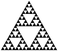
DGIFSs are one of the most general categories of dynamical system where a directed graph is used to impose an order in which the associated functions may be applied. If the directed graph has n vertices then the dynamics of a DGIFS always produce a unique n-component set which is known as an attractor. To understand DGIFSs it is helpful to begin by considering some aspects of the dynamics of the Sierpiński triangle, named after the Polish mathematician Waclaw Sierpiński. The Sierpiński triangle is the attractor of a 1-vertex DGIFS (a standard IFS) and so it provides a useful starting point before we go on to describe more general n-vertex DGIFSs with n ≥ 2.
The Sierpiński triangle
Firstly, for the Sierpiński triangle, X = K(ℝ2), which is the set of all non-empty compact subsets of the real plane, ℝ2. A compact set is closed and bounded in ℝ2, see Sutherland's book for the technical definitions. For our purposes it is enough to know that compact sets are (more or less) subsets of the plane which lie within finite areas of it. The important thing about K(ℝ2) is that its elements are themselves sets, even though we may sometimes call them points. In fact any point (x, y) is also in K(ℝ2) but so are the three example sets illustrated in Figure 1. Clearly K(ℝ2) is an enormous set (of sets).

T0

A

B
Figure 1: Three sets in K(ℝ2).
Secondly the function f: K(ℝ2) → K(ℝ2) is of the following form for the Sierpiński triangle
(1) f(A) = f1(A) ∪ f2(A) ∪ f3(A)
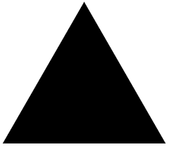
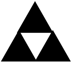
where A is any element in K(ℝ2). Figure 2 shows the effect on T0 of the three separate functions f1, f2 and f3, which together define f. Each of them scales T0 by 0.5 and translates it, no rotations or reflections are involved. After one iteration we obtain
T1 = f(T0) = f1(T0) ∪ f2(T0) ∪ f3(T0).

Figure 2: The first iteration of f defined by f1, f2 and f3.
Just as the Euclidean metric can be used to measure the distance between any two points in the real plane, ℝ2, there is another metric called the Hausdorff metric, named after the German mathematician Felix Hausdorff, which can be used to measure the distance between any two sets in K(ℝ2), (see the books by Barnsley, Falconer, Peitgen et al and Edgar for the definition of the Hausdorff metric). This means, for example, that the Hausdorff metric can measure the distance between the sets A and B in Figure 1. To say f is a contraction mapping means that for any two sets like A and B, the image sets f(A) and f(B) are closer together (with respect to the Hausdorff metric) than A and B are originally. The function f, as defined by Equation (1) and Figure 2, is actually a contraction mapping on K(ℝ2) with respect to the Hausdorff metric. The Contraction Mapping Theorem now ensures that for our dynamical system (K(ℝ2), f), the sequence of iterates or the orbit {f n(A0)} of any starting point A0 always converges to a unique set T in K(ℝ2), which is also the unique fixed point of f, that is f(T) = T. The set T is the fractal known as the Sierpiński triangle. T is also known as the attractor of the IFS because all the orbits of points in K(ℝ2) get closer towards it as we travel along them.
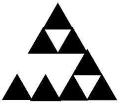
The first 6 points in the orbit {f n(T0)} of T0 under f are illustrated in Figure 3 where we are using a slightly overlapping version of the usual Sierpiński triangle.
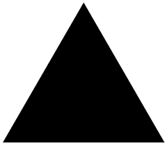
T0 = f 0(T0)
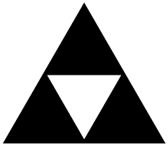
T1 = f(T0) = f 1(T0)
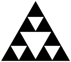
T2 = f(T1) = f 2(T0)
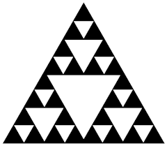
T3 = f(T2) = f 3(T0)
T4 = f(T3) = f 4(T0)

T5 = f(T4) = f 5(T0)
Figure 3: Ti for i = 0 to 5, the first five iterations of the Sierpiński triangle fractal.
We can never draw the Sierpiński triangle but just approximations to it, for example one way is to use points somewhere along an orbit. In fact we don't have to iterate many times before the triangles are of smaller size than the distance between adjacent pixels of any digital image we may be working with.
The machinery behind standard IFSs, like the one that produces the Sierpiński triangle, can be generalised to n-vertex DGIFSs by using the structure of a directed graph. A directed graph is a set of vertices with a set of directed edges that connect vertices to other vertices in specific directions. Functions, contraction mappings like f1, f2 and f3 in Equation (1) above, are assigned to edges in the directed graph which is then used to provide a rule restricting the order in which the functions may be applied. In the simplest case of a standard IFS, which is a DGIFS with a 1-vertex directed graph, where all the edges in the graph are loops, there is no restriction on the order in which the functions may be applied. If the directed graph has n vertices then it can be shown using the Contraction Mapping Theorem that it will have a unique n-component attractor.
A 4-vertex DGIFS based on the Sierpiński triangle
As an example of a DGIFS consider the picture DGIFS5. For this picture the dynamical system is of the form ((K(ℝ2))4, f) where (K(ℝ2))4 = (K(ℝ2), K(ℝ2), K(ℝ2), K(ℝ2)) and f is the overall function made up of the functions f1, f2 and f3 of Figure 2 but applied using the structure of a 4-vertex directed graph (shown in Figure 4). Because f is a contraction (with respect to a metric derived from the Hausdorff metric) the Contraction Mapping Theorem ensures the existence of a unique attractor which is a 4-component set T = (T1, T2, T3, T4) where each Ti is an element of K(ℝ2). Each Ti resembles the Sierpiński triangle T because all the individual mappings used are one of f1, f2 and f3 of Figure 2 as can be seen in Figure 5. In fact the picture labelled DGIFS5 is an illustration of T1.
Now if we put T0 = (T0, T0, T0, T0) = (T0,1, T0,2, T0,3, T0,4) where T0 is the triangle in Figure 3, then the notation for its orbit {f n(T0)} is
T0 = (T0,1, T0,2, T0,3, T0,4)
T1 = f(T0) = (T1,1, T1,2, T1,3, T1,4)
T2 = f(T1) = f2(T0) = (T2,1, T2,2, T2,3, T2,4)
and so on.
As was the case with the Sierpiński triangle, the sequence of iterates or the orbit {f n(A0)} of any starting point A0 = (A0,1, A0,2, A0,3, A0,4) always converges to the attractor T where T is the unique fixed point of f with f(T) = T.

Figure 4: The 4-vertex directed graph used to make the picture DGIFS5.
Figures 4 and 5 illustrate the way the function f is derived from the functions f1, f2 and f3 using a 4-vertex directed graph. Specifically the function f1 is assigned to the edges e1, e4, e7 and e10 in the directed graph of Figure 4. The function f2 is assigned to the edges e2, e5, e8 and e11. The function f3 is assigned to the edges e3, e6 and e9. Just to complicate things further, there is an established convention which requires that the functions map in the opposite direction to the edges they are associated with in the graph. This convention turns out to be useful for the theory but means for example that the edge e1 goes from the vertex v1 to v4 in Figure 4 but the function f1 maps from the vertex v4 to v1 in Figure 5.

Figure 5: The first iteration of f which uses the 4-vertex directed graph of Figure 4.
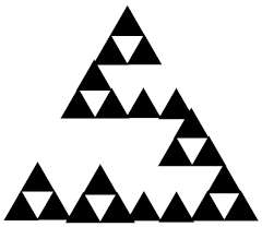
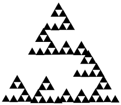
The first components Ti,1, for i = 0 to 5, of the first 5 iterations of T0 are shown in Figure 6, where the functions f1, f2 and f3 have been modified a little for use in the directed graph by occasionally adding in some very small translational offsets and very slightly changing the scaling factor of 0.5.
T0,1
T1,1
T2,1
T3,1
T4,1

T5,1
Figure 6: Ti,1 for i = 0 to 5, the first five iterations of the first fractal component of the attractor of a 4-vertex DGIFS.
Comparing Figure 6 to Figure 3, even though the individual mappings are (almost) exactly the same, the effect of the imposed directed graph is to break up the symmetry of the original Sierpiński triangle.
The following is a list of all the pictures in the DGIFS category. The pictures Cloud 7, DGIFS7c, DGIFS7d and DGIFS11a are pictures of components of 2-vertex DGIFS attractors. Static 1, Static 2, Static 3 and Strings are components of 3-vertex DGIFS attractors. The picture labelled DGIFS5 is a component of the attractor of a 4-vertex DGIFS, closely related to the Sierpiński triangle, as described above. Light on a Lake, DGIFS8b, Intersection, Red City, Ruins and Light over Waterloo are components of 5-vertex DGIFS attractors.
Other pictures that use a directed graph in much the same way as described above, that is to restrict the order in which the associated functions are applied, are Veiled Grid (made with trigonometric functions) and Planetary Disk, Planetary Disk 2, Lunar Disk and K Disk (made with Möbius transformations).
Music videos – high resolution fractal animations
Three fractal music videos created using DGIFSs are on YouTube.
One is an animation (4m 08s) of the picture Light on a Lake in both a 1080p version and a 4K version. The piano soundtrack is “An Amalgamation Waltz 1839” by Joep Beving.
Another is an animation (5m) of the picture Red City which is also in both a 1080p version and a 4K version. The soundtrack “Red City Moves” (piano and strings) is available on some music streaming services.
The third is “Circular Strings”, an animation (4m) based on the pictures Strings, Static 1, Static 2, and DGIFS11a, available in both a 1080p version and a 4K version. The soundtrack is the guitar instrumental “Circular Strings” which is available on some music streaming services.
Any individual frame of these animations can be made into a fine art print.
References
The following research proves that we can expect DGIFSs generally to give us something different and new when compared to standard IFSs. These results provided the motivation to create the pictures of the DGIFS fractals which can be found in the gallery.
G. C. Boore, Directed Graph Iterated Function Systems, Ph.D. thesis, School of Mathematics and Statistics, St Andrews University, (2011).
G. C. Boore, Some new classes of directed graph IFSs, (2014).
G. C. Boore and K. J. Falconer, Attractors of directed graph IFSs that are not standard IFS attractors and their Hausdorff measure, Math. Proc. Camb. Phil. Soc. 154 (2013), 324-349.
This textbook describes the mathematics of a DGIFS and a standard (1-vertex) IFS. (For DGIFSs see Section 4.3 and Chapter 6, where the directed graph is called a Mauldin-Williams graph after R. D. Mauldin and S. C. Williams who gave a definitive description of DGIFSs in n-dimensional Euclidean space. They also calculated their Hausdorff dimension, assuming a separation condition holds.)
G. A. Edgar, Measure, Topology, and Fractal Geometry, Springer-Verlag, New York, 2nd Ed. (2000).
Graeme Boore's articles on arXiv include the following article, which proves results about directed graph self-similar measures, where the corresponding DGIFSs are defined on n-dimensional Euclidean space and satisfy the Open Set Condition. The proof uses an application of the Renewal Theorem and the results obtained have applications in the area of multifractal analysis.
G. C. Boore, The qth packing moments and the packing Lq-spectra of directed graph self-similar measures, (2017).