- pictures and mathem- atics
- dynamical systems
- the real plane
- trigono- metric functions (T)
- complex dynamics (CD)
- directed graph iterated function systems (DGIFSs)
Making pictures with trigonometric functions
The pictures in the T (trigonometric functions) category that can be found in the gallery are of dynamical systems (X, f) where X is the real plane and f : X → X is a function based on the composition of trigonometric functions with low-degree polynomials. The function f takes the form
f(x, y) = (x, y) + h × (p(x, y), q(x, y))
where p and q are functions which map points in the real plane ℝ2 to single values on the real line ℝ and involve the composition of the trigonometric functions sine and cosine with low-degree polynomials in the variables x and y. The function f makes use of the vector space properties of the real plane, with the addition of vectors and the multiplication by the step-size h.
Once co-ordinates have been assigned to the left, right, top and bottom of a digital image, the step-size h is usually chosen to be smaller than the distance between adjacent pixels. This means that on iterating f we obtain orbits which map out (approximately) continuous smooth paths in the resulting digital image. These paths are present in all the pictures in the T category as the familiar waves and spirals associated with the trigonometric functions sine and cosine.
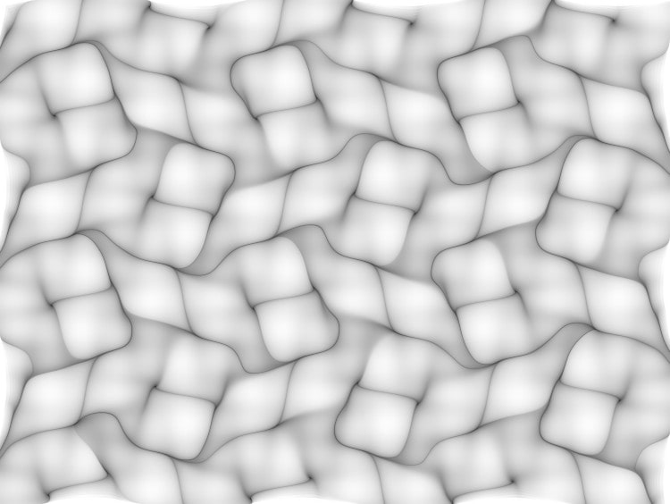
As a specific example the picture in Figure 1 has the co-ordinates: left = −10, right = 10, top = 8, bottom = −8. The step-size is h = 0.1 and the image size is 720 × 540 pixels. In the function f above, the functions p and q are
p(x, y) = −cos(y + cos(πx))
q(x, y) = cos(x + cos(πy)).
Using random orbits of length 50, the pixels have been coloured by counting the number of times they are landed on by an orbit.

Figure 1: Example of a picture in the T category, made with trigonometric functions.
Pictures in the T category are Pebble Spiral 1, Pebble Spiral 2, Sand Flow, Optical, Veiled Grid, Seascape, Unicorn, T1a, T3 and T9a.
The picture Veiled Grid is the result of an experiment to see what happens if we restrict the order of the functions being applied by using a 2-vertex directed graph with probabilities. The functions and probabilities are assigned to the edges in the directed graph. We travel from one vertex to another using an edge which is decided upon by using a random number generator and the probabilities associated with the edges. This idea is similar to the way that a directed graph is used in directed graph iterated function systems.
References
Information about this type of dynamical system can be found in Chapter 14 of the following book.
C. A. Pickover, Computers, Pattern, Chaos, and Beauty, Dover, New York, (2001).